Introduction

Hyperspectral images have the ability to see what the human eye cannot see, but what truly turns data into information and extracts features from noise is spectral preprocessing and dimensionality reduction. In this issue, we use the most intuitive case - bruised kiwifruit, to show you how the original spectrum gradually reveals clear tissue structure and damage characteristics under a series of preprocessing (smoothing, SNV, MSC) and dimensionality reduction methods (PCA, MNF). With just a few images, you can see the huge difference before and after hyperspectral processing, and quickly understand why preprocessing is more important than modeling itself.

4 Spectral image preprocessing

4.1 Spectral preprocessing

The smoothing method is mainly used to eliminate high-frequency random noise in the spectrum, while preserving the overall trend and peak shape of the spectrum as much as possible.

(1) Moving average

Moving average is the most basic smoothing method. It smooths the spectrum by taking the average of the current point and its neighboring points. This method can smooth high-frequency noise, but is not sensitive to some sharp noise. The formula is as follows:

Among them, is the size of the moving window.

Python code example:

(2) Savitzky Golay Smooth

The core idea of SG smoothing is to perform polynomial fitting on spectral signals within a sliding window, and replace the original spectral points with the fitted values. Compared with simple moving averages, SG smoothing can not only remove high-frequency noise, but also maintain the spectral peak shape and local features of the signal. The formula is as follows: When the window size is 2m+Under the condition of 1, for theiThe smoothness of a spectral point is:

Among them, is the coefficient obtained by polynomial fitting, which is the original value of the spectral points within the window.

Python code example:

(3) Median filtering

Median filtering replaces the current point value with the median within the window, which is particularly effective for occasional spiky noise (spikes).

Python code example:

(4) Standard Normal Transformation (SNV)

SNV is a normalization method that eliminates scattering effects or intensity differences between spectra by centralizing and standardizing each spectrum, while preserving the relative morphology of the spectra. The formula is as follows:

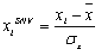
Among them, represents the spectral mean and represents the spectral standard deviation.

Python code example:

(5) Multivariate Scattering Correction (MSC)

MSC fits each spectrum to a reference spectrum (usually an average spectrum) through linear regression, correcting for multiplicative and additive scattering effects. This method can correct the intensity differences caused by scattering and preserve the shape characteristics of the spectrum. The formula is as follows: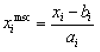Among them

Among them, is theiThe wavelength spectrum, reference spectrum, is usually the average spectrum of all samples, and is the regression coefficient, which is the fitted spectrum.

Python code example:

4.2 Spectral Image Dimensionality Reduction

(1) Principal Component Analysis Dimensionality Reduction (PCA)

PCA is a commonly used dimensionality reduction method in hyperspectral image processing, used to reduce band redundancy, reduce noise, and extract primary spectral information. Hyperspectral images are typically represented by three-dimensional data cubes, containing spatial dimensions and hundreds of spectral bands. The core idea of PCA dimensionality reduction is to treat the spectral vector of each pixel as high-dimensional data, and to obtain principal components sorted by variance size by performing zero mean transformation on all pixel data, calculating the covariance matrix, and computing their eigenvalues and eigenvectors. Selecting the first few principal components can map hyperspectral data from high-dimensional to low dimensional, while retaining most of the spectral information. The reduced dimensional data not only reduces computational complexity, but also significantly improves signal-to-noise ratio, making it suitable for visualization, classification, or clustering analysis. For example, the first three principal components can be combined to create a pseudo color image that visually displays spatial structure. Overall, PCA dimensionality reduction is an important preprocessing method in hyperspectral image processing and analysis, which can effectively compress data, remove redundancy and noise, while preserving spectral features.

(2) Minimum noise fraction dimensionality reduction (MNF)

In hyperspectral image processing, MNF dimensionality reduction is a commonly used data denoising and compression method, whose core idea is to extract the main signal components by considering the spectral noise characteristics. MNF dimensionality reduction is generally carried out in two steps: * Step 1, noise estimation is performed on the original hyperspectral data and noise normalization is performed on the data to standardize the impact of noise; The second step is to perform principal component analysis (PCA) on the normalized data, extracting the components with high variance as the main signals and discarding the low variance components dominated by noise. Unlike traditional PCA, MNF considers the noise structure first, making the first few principal components after dimensionality reduction better in signal-to-noise ratio and better able to highlight the true spectral signal. The data reduced by MNF not only reduces band redundancy but also effectively reduces noise, making it widely used in tasks such as visualization, classification, and target recognition of hyperspectral images. Due to its ability to simultaneously achieve noise suppression and feature compression, MNF is often considered an advanced dimensionality reduction method for processing hyperspectral data.

4.4 Comparison before and after the case

(1) Spectral preprocessing case

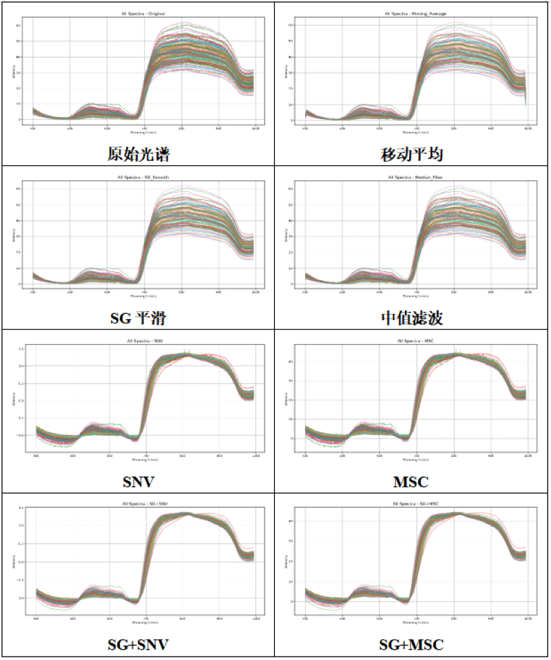
The spectral curves processed by different preprocessing methods are shown in the following figure. Compared to the original spectrum, smoothing preprocessing methods such as Savitzky Golay, moving average, and median filtering mainly eliminate high-frequency fluctuations on the spectral curve, making the spectral curve smoother while maintaining the basic shape of the overall peak position and baseline. The SNV method standardizes the amplitude and offset of the original spectrum, aligning the spectra of different samples at the same level while slightly altering the overall height of the curve. MSC corrects the amplitude and offset differences caused by light scattering through linear regression, while maintaining peak shape characteristics and eliminating scattering differences between samples. However, SNV and MSC did not eliminate high-frequency noise in the spectrum. The combination method (such as SG+SNV or SG+MSC) first smooths the spectrum with high-frequency noise, and then performs scattering correction, balancing the effects of smoothing and scattering correction to make the spectrum both flat and maintain peak shape characteristics. By comparing the spectra before and after processing, it is possible to intuitively observe the adjustment effects of various methods on noise, scattering, and baseline, and thus select the most suitable preprocessing strategy.

(2) Spectral Image Dimensionality Reduction Case

Taking the spectral image dimensionality reduction of bruised kiwifruit as an example, the hyperspectral image and specific wavelength grayscale image of bruised kiwifruit are shown in the following figure.

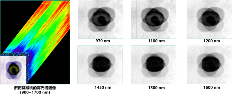
Hyperspectral image and specific wavelength grayscale image of bruised kiwifruit

After conducting PCA and MNF analysis on the hyperspectral data of bruised kiwifruit, it was found that both methods were able to extract features related to tissue changes in the principal components, but there were significant differences in their performance. The PC1 of PCA mainly characterizes the overall reflectance and density distribution of fruit pulp tissue. PC2 can significantly highlight the absorption enhancement in the bruised area and is the most diagnostic component in PCA; Starting from PC3, noise dominates and obvious stripe artifacts appear, which is no longer suitable for further analysis. In contrast, MNF effectively suppresses noise by sorting according to signal-to-noise ratio. Its MNF1 exhibits stable tissue background features, MNF2 can separate the core area of bruising with higher contrast and clearer boundaries, and MNF3 further strengthens the damaged edge structure, presenting a hierarchical change in bruising diffusion. Overall, MNF is significantly superior to PCA in enhancing bruising features, suppressing noise, and preserving tissue details, with MNF2-MNF3 being the most valuable diagnostic feature components.

PCA and MNF analysis of full spectrum images of kiwifruit samples

Next episode preview

In the next issue, we will introduce the recognition and classification of hyperspectral images, as well as the supervised classification methods for hyperspectral image classification.